Scaling Laws for Optimal LR and Batch Size - Part VI

Akima spline interpolation

Introduction

In the previous post in this series, I discussed how the fit from Part III gave a learning rate forecast with room for improvement. Working on resolving that will take some time for the experiments to run on my hardware, so check back in about two weeks. I will have plenty of other experiments running and posts in the meantime!

Anyway, I found myself revisiting the hyperparameter scaling laws from Porian et al., 2024. While these scaling laws are fit in terms of model parameter count N only, the authors use an intriguing method—Akima spline interpolation—to obtain a regression targets for the optimal batch size and learning rate beyond the granularity of their actual sweeps.

In this post, we will see about using Akima spline interpolation as well, using the data I already collected in Part III. I am interested to see if it meaningfully changes our hyperparameter scaling laws and also if it allows the scaling laws to remain approximately intact if I artificially reduce the granularity of the (B, \eta) grid.

Implementation Plan

Instead of implementing Akima spline interpolation from scratch, I will use the SciPy implementation of scipy.interpolate.Akima1DInterpolator (docs here).

This method is only supported for 1D interpolation, so to obtain an interpolated 2D grid I will first interpolate the (\eta, loss) pairs independently for each batch size B, and then evaluate the interpolation at a higher-granularity mesh of learning rates \eta. Then, I will take the new points, interpolate (B, loss) for each LR \eta independently, and then evaluate the interpolation at a higher-granularity mesh of batch sizes B.

This will result in a 2D (batch size, learning rate) mesh grid with both dimensions having increased granularity compared to what they started with. From there I can take the minimum predicted loss and use the associated learning rate and batch size as regression targets for the scaling law, which I will refit.

Implementation

Here is some minimal code implementing this logic:

def build_interpolated_df(df, n_lr_interp=13, n_bs_interp=7):
  from scipy.interpolate import Akima1DInterpolator

  df2 = pd.DataFrame()
  model_sizes = df["N"].unique()
  data_sizes = df["D"].unique()
  batch_sizes = df["B"].unique()
  for n in model_sizes:
    for d in data_sizes:
      for b in batch_sizes:
        filtered = df[(df["N"] == n) & (df["D"] == d) & (df["B"] == b)].sort_values(by="E")
        x = np.log2(filtered["E"]).to_numpy()
        y = np.log2(filtered["Loss"]).to_numpy()
        akima = Akima1DInterpolator(x, y, method="akima")
        x_highres = np.linspace(start=-13, stop=-7, num=n_lr_interp)
        y_highres = akima(x_highres)
        df_temp = pd.DataFrame()
        df_temp["N"] = np.full_like(x_highres, fill_value=n)
        df_temp["D"] = np.full_like(x_highres, fill_value=d)
        df_temp["B"] = np.full_like(x_highres, fill_value=b)
        df_temp["E"] = np.pow(2, x_highres)
        df_temp["Loss"] = np.pow(2, y_highres)
        df2 = pd.concat([df2, df_temp])
  df2 = df2.reset_index()

  df3 = pd.DataFrame()
  model_sizes = df2["N"].unique()
  data_sizes = df2["D"].unique()
  learning_rates = df2["E"].unique()
  for n in model_sizes:
    for d in data_sizes:
      for e in learning_rates:
        filtered = df2[(df2["N"] == n) & (df2["D"] == d) & (df2["E"] == e)].sort_values(by="B")
        x = np.log2(filtered["B"]).to_numpy()
        y = np.log2(filtered["Loss"]).to_numpy()
        akima = Akima1DInterpolator(x, y, method="akima")
        x_highres = np.linspace(start=15, stop=21, num=n_bs_interp)
        y_highres = akima(x_highres)
        df_temp = pd.DataFrame()
        df_temp["N"] = np.full_like(x_highres, fill_value=n)
        df_temp["D"] = np.full_like(x_highres, fill_value=d)
        df_temp["E"] = np.full_like(x_highres, fill_value=e)
        df_temp["B"] = np.pow(2, x_highres)
        df_temp["Loss"] = np.pow(2, y_highres)
        df3 = pd.concat([df3, df_temp])
  df3 = df3.reset_index()

  return df3

Since bootstrapping didn’t make a substantial difference in the fits earlier, for simplicity I will omit it from the fits in this post.

Visualization

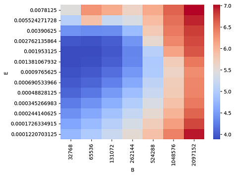
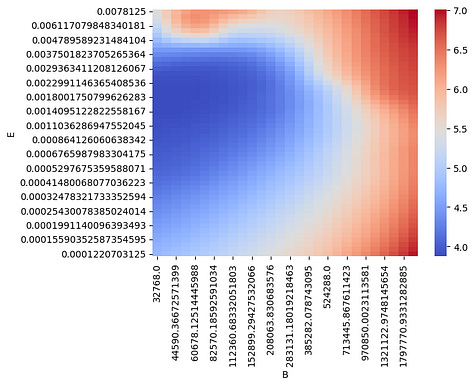
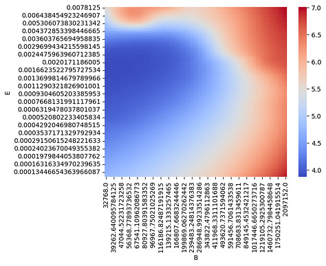
Here is a visualization of the loss surface for a particular model, data size pair (N, D). On the left is the original loss surface w.r.t. (B, \eta), and on the middle and right are Akima spline interpolations viewed at increasing granularities.

Sanity Check

First as a sanity check, we’ll set the (B, \eta) mesh grid to be the exact same one we start with—in other words, for the moment we will only evaluate the splines at the points they were trained on. For the non-smoothing splines we’re using, this should give the exact same result when we fit our scaling laws. Let’s see.

import statsmodels.api as sm
import pandas as pd
import numpy as np

def fit_scaling_law(df):
    optimum_rows = df.loc[df.groupby(['N', 'D'])['Loss'].idxmin()]
    optimum_rows = optimum_rows.sort_index()

    endog = np.log2(optimum_rows[['B']])
    exog = sm.add_constant(np.log2(optimum_rows[['D']]))
    model = sm.OLS(endog, exog)
    results = model.fit()
    p1 = results.params

    endog = np.log2(optimum_rows[['E']])
    exog = sm.add_constant(np.log2(optimum_rows[['N', 'D']]))
    model = sm.OLS(endog, exog)
    results = model.fit()
    p2 = results.params
    return (p1, p2)

In this case, we do indeed get the exact same fit for both df and build_interpolated_df(df).

New Fit

Now let’s increase the mesh grid granularity by 10x for both the learning rate and batch size and reexamine the fit. In code:

interpolated = build_interpolated_df(
    df, n_lr_interp=130, n_bs_interp=70
)
fit_scaling_law(interpolated)

We obtain a fit of

\(B^{*} = 0.269 D^{0.640}\)

\(\eta^{*} = 0.078N^{-0.490}D^{0.264}\)

Test Point

Plugging in our test point (N, D) = (4.7B, 100B), we have

\(B^{*} = 0.269 * (2^{21} * 50,000)^{0.640} = 3,040,438\)

\(\eta^{*} = 0.078 * (13 * 128 * 128 * 28^3)^{-0.490} * (2^{21} * 50000)^{0.264} = 0.00115694485\)

The optimal batch size has changed from 2M to 3M thanks to Akima interpolation on the training data, but the optimal learning rate is now 0.001 instead of 0.0009, which is not much different and in fact went the wrong way from the ground-truth LR optimum of ~0.0002 at batch size 2M.

This suggests our optimum learning rate forecast must be fixed via other means: using Akima interpolation to remove quantization artifacts from the regression targets isn’t doing much for the learning rate scaling law. On the other hand, we saw that Akima interpolation was helpful for the batch size forecast and resulted in some meaningful improvements there.

Artificial Coarsening

We saw that Akima interpolation wasn’t helpful with our current LR granularity, but let’s test if it is helpful when every other (half) of the learning rates are missing.

Here’s some code implementing this:

def artifically_coarsen_lr(df):
    learning_rates = sorted(df["E"].unique().tolist())
    learning_rates = set(learning_rates[::2])
    new_df = df[df["E"] in learning_rates]
    new_df = new_df.reset_index()
    return new_df

coarsened = artifically_coarsen_lr(df)
interpolated = build_interpolated_df(
    coarsened, n_lr_interp=130, n_bs_interp=70
)
fit_scaling_law(interpolated)

And we obtain a fit of

\(B^{*} = 0.207 D^{0.654}\)

\(\eta^{*} = 0.099 N^{-0.458}D^{0.217}\)

which is fairly close to what we had when applying Akima interpolation without coarsening first. The only noticeable difference is the dataset exponent for learning rate, which is a bit smaller than the 0.264 seen above.

Now let’s try with coarsening and without Akima interpolation:

coarsened = artifically_coarsen_lr(df)
fit_scaling_law(coarsened)

In this case, the dataset exponent for the batch size scaling law drops to 0.480, even falling below the value in Part III. Meanwhile, the model size exponent drops to -0.533, far from the approximate -0.45 to -0.49 seen here. It seems Akima interpolation is helpful when the learning rate is coarse.

Automatic Pruning of Irrelevant Variables

One other interesting thing I noticed is that if I specify a full power law for batch size and learning rate in terms of model size and dataset size—instead of the batch size just depending on dataset size—then using Akima spline interpolation empirically prunes away the irrelevant variable (model size). Let’s take a look:

def fit_scaling_law_full(df):
    optimum_rows = get_optimum_rows(df)

    endog = np.log2(optimum_rows[['B']])
    exog = sm.add_constant(np.log2(optimum_rows[['N', 'D']]))
    model = sm.OLS(endog, exog)
    results = model.fit()
    p1 = results.params

    endog = np.log2(optimum_rows[['E']])
    exog = sm.add_constant(np.log2(optimum_rows[['N', 'D']]))
    model = sm.OLS(endog, exog)
    results = model.fit()
    p2 = results.params
    return (p1, p2)

interpolated = build_interpolated_df(
    df, n_lr_interp=130, n_bs_interp=70
)
fit_scaling_law_full(interpolated)

The result is

\(B^{*} = 0.240 N^{0.006} D^{0.640}\)

\(\eta^{*} = 0.078N^{-0.490}D^{0.264}\)

as you can see, it is remarkably clean in terms of how close to zero the model size exponent is, for the batch size scaling law.

Conclusion

In this post, I used Akima spline interpolation to create synthetic data for the hyperparameter scaling laws. This led to meaningful alterations of the batch size, suggesting our sweep may benefit from a finer grid. When reducing the granularity of the learning rate sweep artificially, the interpolation also resulted in meaningful improvements compared to a naive OLS fit to the coarse grid optima. Finally, when restoring model size as a regressor for the batch size scaling law, fitting the power law after running Akima interpolation led to a near-zero exponent for this empirically-irrelevant variable.