Scaling Laws for Optimal LR and Batch Size - Part III

Sweep granularity matters

Introduction

Welcome back.

In Part I and Part II of this series, I fit scaling laws for optimal batch size B^* and optimal learning rate \eta^*, but found that the data scaling exponent differed from the StepFun paper, Li et al., 2025.

In Part IIb, I identified insufficient learning rate granularity as a possible culprit for the poor fit. In this post, I will upgrade the learning rate granularity to equal that of the Li et al., 2025.

Experiment Planning

I will start over with data collection, this time using grid data only. I will use n_layer = 6, 8, 12, 16, 24 as before, and generate N = 13 * 128^2 * n_layer^3 as before.¹ I will use dataset sizes 128M, 256M, 512M, 1024M.

I will use batch sizes in powers of two between 32768 and 2097152 tokens, and learning rates in powers of 2^0.5 from 0.0078125 to 0.0001220703125, yielding G=91 grid points.

The total compute expenditure in FLOPs is

\(6 \big{(}\sum_{i} N_{i}\big{)} \big{(}\sum_{j} D_{j}\big{)} G \approx 4.5 \cdot 10^{21}\)

which is ~5x larger than the prior experiments and just over 10% of compute required to train LLaMA-1-7B. There are over 1800 runs in total.

Experiment Data

The data for the optimal (B, \eta) pairs is

               N           D       B         E      Loss
86      46006272   127991808   32768  0.001953  3.880559
175    109051904   127991808   32768  0.000977  3.794820
252    368050176   127991808   65536  0.000691  3.714983
346     46006272   255983616   65536  0.001953  3.682230
436    109051904   255983616   65536  0.001381  3.582214
526    368050176   255983616   65536  0.000977  3.486761
620     46006272   511967232   65536  0.002762  3.518618
697    109051904   511967232  131072  0.001953  3.403666
786    368050176   511967232  131072  0.000977  3.287104
881     46006272  1023934464  131072  0.003906  3.384921
970    109051904  1023934464  131072  0.001953  3.256896
1059   368050176  1023934464  131072  0.000977  3.123393
1161   872415232   127991808   65536  0.000488  3.670941
1252   872415232   255983616   65536  0.000488  3.434034
1331   872415232   511967232  131072  0.000691  3.233707
1445  2944401408   127991808   32768  0.000244  3.611588
1524  2944401408   255983616   65536  0.000345  3.371229
1604   872415232  1023934464  131072  0.000691  3.058425
1693  2944401408   511967232  131072  0.000345  3.160028
1784  2944401408  1023934464  131072  0.000345  2.977672

Fitted Scaling Law

Using the complete set of (N, D) pairs, the bootstrapped parameter-averaged fit is:

\(B^{*} = 1.27 D^{0.561}\)

\(\eta^{*} = 0.118 N^{-0.489} D^{0.241}\)

which is fairly close to the dataset exponents in the StepFun paper, Li et al., 2025, which were 0.571 and 0.307, respectively.

The difference in batch size proportionality constant can be attributed to a different tokenizer and dataset—I used the T5 tokenizer and the C4 dataset. The difference in the learning rate proportionality constant and parameter exponent can be attributed to the locked aspect ratio for my models.²

Visualizations

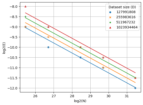
Next, we’ll recreate the visualizations in Figure 6 of the StepFun paper. The fitted scaling law for learning rate as a function of dataset size D is plotted below:

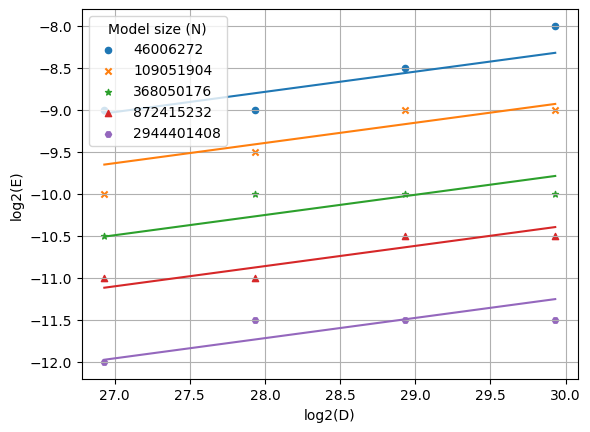
I also plotted the fitted scaling law for learning rate as a function of model size N:

Summary

In this post, I ran over 1,800 experiments and obtained the optimal (B, \eta) for each of twenty (N, D) pairs. I fit the scaling laws for optimal batch size and optimal learning rate, and I approximately recovered the data scaling exponents from Li et al., 2025. Lastly, I plotted the scaling law and recovered figures similar to Figure 6 of Li et al.

1. I use SwiGLU with d_ff = 3 * d_model and d_model = 128 * n_layer as before.

2. In other words, the ratio d_model/n_layer is constant, which impacts the fit.